21. TML Simulator

TML_simulator: The World’s Fastest First‑Principles Carryover Engine with Direct SCADA/DCS Integration and Real-Time Machine Learning, AI, Agentic AI

Tip

You can also view the TML Simulator FAQ
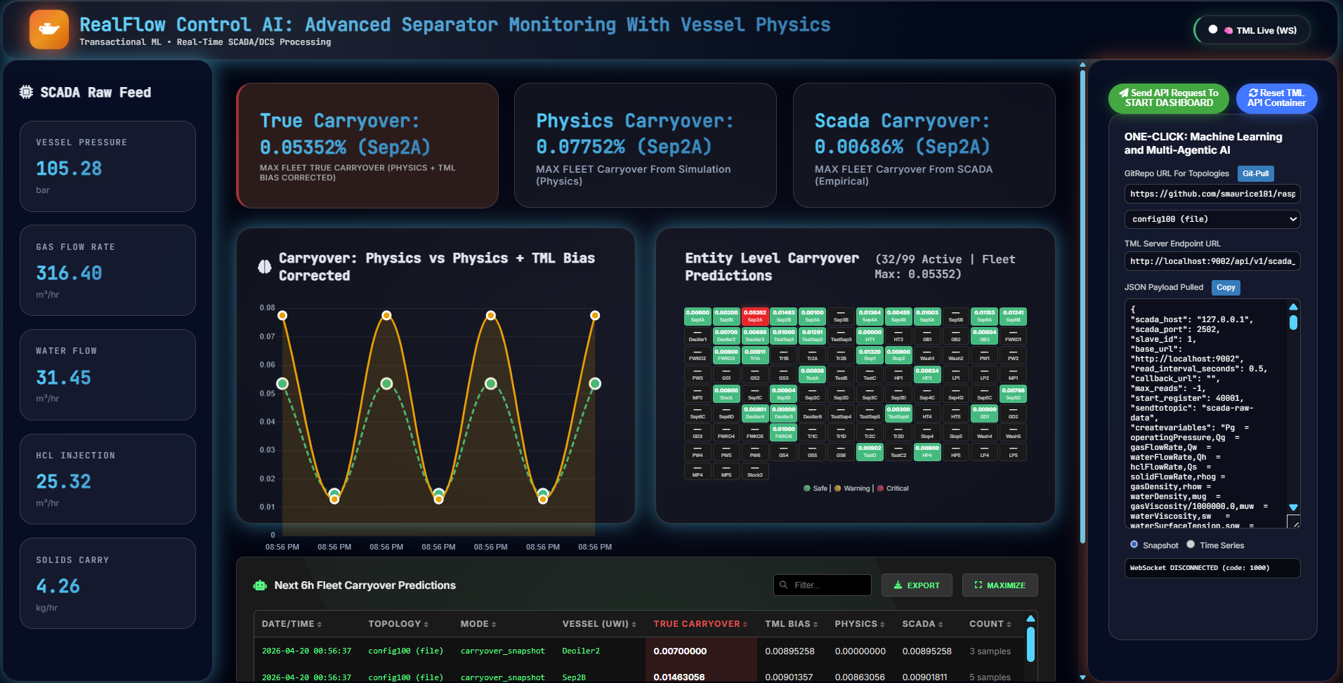
RealFlow Control AI: Dashboard (Main dashboard for running the entire solution)
To use the RealFlow Dashboard, you need to run the TML Server docker container

21.1. Executive Summary

TML_simulator is a first‑principles physics engine that computes liquid‑carryover risk per vessel in under **1 milliseconds per snapshot while remaining fully auditable, equation‑driven, and SCADA‑ready. Built on Souders‑Brown‑based droplet‑physics and Numba‑accelerated computation, it:

Runs real‑time physics‑baseline snapshots at SCADA clock‑speed
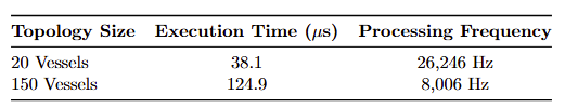
To validate enterprise readiness, 150-vessel fleets were executed at 8,006 Hz.
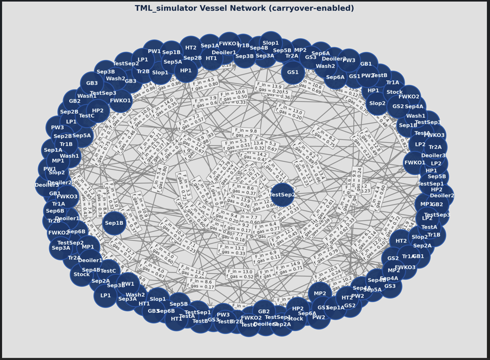
This speed enables Network Topology Convergence, allowing the simulator to perform multiple “internal iterations” of the entire plant’s physics for every single sensor update received. Below is a 20 and 150 vessel (see Appendix D below: Vessel 20 and Vessel 150) simulation
The 8,006 Hz benchmark achieved for a 150-vessel fleet is not merely a speed metric; it is a functional requirement for Level 5 Autonomy. In a standard 100ms SCADA clock cycle, the TML Simulator completes 800 full internal iterations of the plant’s physics. This “Velocity

6 Headroom” allows the system to perform real-time sensitivity auditing—simulating hundreds of “What-If” scenarios (e.g., “What if the pressure spikes 5% in Vessel A?”) before the next sensor update even arrives.

Generates offline‑ready, time‑series physics data for ML, digital twins, and alarm‑tuning,
NO PI Historian is needed for the Machine Learning and AI – all physics, processing, machine learning, AI, Agentic AI handled by TML solution Dashboard: See Appendix E: TML RealFlow Solution
Is config‑driven, not hard‑coded, so it can be reused across any separation‑train topology.

Unlike black‑box AI or heavy‑CFD‑style tools, TML_simulator is focused‑physics code: it does one thing cleanly — predict carryover bias — and integrates that insight into control‑systems, dashboards, and ML‑bias layers above.

21.2. Why TML Simulator Is Industry‑Leading

Most “best‑in‑class” simulation technologies fall into two camps:

Full‑dynamic, multi‑phase simulators — physically rich, but too slow and too complex for SCADA‑integration and real‑time monitoring.
Pure‑data ML models — fast, but opaque, statistically fragile, and hard to defend in design‑reviews or audits.

TML_simulator occupies a third, superior tier:

It respects real‑world physics (Souders‑Brown, droplet‑settling, mist‑pad efficiency, gravity‑chamber performance).
It runs at SCADA‑clock‑speed (snapshot mode), enabling continuous “physics‑baseline” monitoring inside existing control systems.
It produces training‑data and offline‑time‑series for ML and digital twins, without forcing a trade‑off between “physics” and “speed”.

As a result, TML_simulator is:

More interpretable than any pure‑data ML tool,
Faster and lighter than any full‑multi‑phase‑dynamic simulator,
More production‑ready than either, because it can run inside the same SCADA environments where operators actually make decisions.

21.3. TML Simulator Can Process

These are the vessels TML simulator can process:

separator

fwko

tank

scrubber

ko_drum

dehydrator

Default Values for Reference:

“separator”: {“diameter”: 3.5, “height”: 12.0, “gravity_h”: 2.5, “mist_eff”: 0.98, “souders_k”: 0.35, “d_mean_um”: 220.0, “carryover_scale”: 0.1},

“fwko”: {“diameter”: 2.8, “height”: 8.0, “gravity_h”: 2.0, “mist_eff”: 0.95, “souders_k”: 0.32, “d_mean_um”: 300.0, “carryover_scale”: 0.1},

“tank”: {“diameter”: 5.0, “height”: 15.0, “gravity_h”: 4.0, “mist_eff”: 0.85, “souders_k”: 0.25, “d_mean_um”: 500.0, “carryover_scale”: 0.1},

“scrubber”: {“diameter”: 2.2, “height”: 7.0, “gravity_h”: 1.8, “mist_eff”: 0.99, “souders_k”: 0.35, “d_mean_um”: 150.0, “carryover_scale”: 0.05},

“ko_drum”: {“diameter”: 2.0, “height”: 6.0, “gravity_h”: 1.6, “mist_eff”: 0.80, “souders_k”: 0.28, “d_mean_um”: 400.0, “carryover_scale”: 0.15},

“dehydrator”: {“diameter”: 3.0, “height”: 10.0, “gravity_h”: 2.2, “mist_eff”: 0.99, “souders_k”: 0.38, “d_mean_um”: 100.0, “carryover_scale”: 0.02}

21.4. The Fundamental Physics / Math

TML_simulator is built on equation‑driven separation physics that mirrors real‑world separation‑design practice. The core ideas are:

21.4.1. 1. Gas‑Velocity versus Souders‑Brown Limit

For each vessel, the cross‑sectional area and gas‑velocity are computed from geometry and flow:

\[A_{i} = \pi\left( \frac{D_{i}}{2} \right)^{2},q_{g,i} = \sum_{j}^{}F_{g,ji} \cdot h_{u,j},u_{g,i} = \frac{q_{g,i}}{A_{i} \cdot H_{i}}\]

where:

\(A_{i}\): vessel cross‑sectional area,
\(D_{i}\): diameter, \(H_{i}\): height,
\(q_{g,i}\): effective gas‑flow through the vessel (weighted by upstream holdup‑fractions \(h_{u}\)).

The Souders‑Brown limiting velocity is:

\[v_{S,i} = K_{i}\sqrt{\frac{\rho_{L,i} - \rho_{G,i}}{\rho_{G,i}}}\]

\(K_{i}\): vessel‑specific Souders‑Brown constant,
\(\rho_{L,i},\rho_{G,i}\): liquid and gas densities.

Mist‑loading (dimensionless gas‑velocity ratio):

\[\left. \ \phi_{u,i} = \frac{u_{g,i}}{v_{S,i}} \in (0,5) \right\rbrack\]

Mist‑pad capture efficiency:

\[\eta_{\text{mist},i}(\phi_{u,i}) = \eta_{m,i} \cdot \frac{\phi_{u,i}}{5}\]

\(\eta_{m,i}\): maximum mist‑pad efficiency.

21.4.2. 2. Droplet‑Settling in the Gravity Section

The engine models a log‑normal droplet‑size distribution:

\[\ln d \sim \mathcal{N(}\mu = \ln d_{\text{mean}},\text{ }\sigma = \ln d_{\text{sigma}})\]

At each 3‑point quadrature point \(z_{j} \in \{ - 1.2,0.0,1.2\}\)with weight \(w_{j} \in \{ 0.25,0.5,0.25\}\), the droplet diameter is:

\[d_{j} = d_{\text{mean}} \cdot \exp(z_{j} \cdot \ln d_{\text{sigma}})\]

Stokes‑regime terminal‑settle velocity:

\[v_{s,j} = \frac{(\rho_{L,i} - \rho_{G,i})gd_{j}^{2}}{18\mu_{G,i}}\]

Dimensionless settling‑number:

\[\left. \ \text{Stn}_{j} = \frac{v_{s,j} \cdot h_{g,i}}{u_{g,i} \cdot H_{i}} \in (0,15 \right\rbrack\]

(capped at 15, as in standard separation‑design practice).

Droplet‑capture fraction in the gravity section:

\[E_{\text{gravity},j} = 1 - \exp( - \text{Stn}_{j})\]

Total capture fraction:

\[E_{T} = 1 - (1 - \eta_{\text{inlet}})(1 - E_{\text{gravity},j})(1 - \eta_{\text{mist},i})\]

\(\eta_{\text{inlet}}\): inlet‑device efficiency.
\(E_{\text{gravity},j}\): droplet‑capture in the gravity section.
\(\eta_{\text{mist},i}\): mist‑pad capture.

Droplet‑escape (carryover) at each point:

\[\mathcal{F}_{\text{esc},j} = 1 - E_{T}\]

Quadrature‑averaged droplet‑carryover:

\[C_{i} = \sum_{j}^{}w_{j} \cdot \mathcal{F}_{\text{esc},j}\]

Carryover percentage:

\[\text{carryover}_{i}(t) = 100 \cdot C_{i} \cdot \text{carryover_scale}_{i}\]

21.4.3. 3. Vessel‑Holdup and Time‑Stepping

Liquid holdup evolves according to:

\[\frac{dV_{i}}{dt} = - C_{i} \cdot q_{l,i}\]

\(q_{l,i} = \sum_{j}^{}F_{l,ji} \cdot h_{u,j}\): total liquid‑in‑flow,
\(V_{i}\): liquid volume in the vessel.

Discretized via forward‑Euler:

\[V_{i}(t) = \max\left( V_{i}(t - \Delta t) + \frac{dV_{i}}{dt} \cdot \Delta t,\text{:,}0 \right)\]

which is exactly what the inner‑loop of physics_carryover computes.

21.4.4. Why This Is Production‑Grade

TML_simulator is production‑physics, not a toy:

It runs sub‑10‑ms snapshots per SCADA cycle, giving a physics‑baseline carryover‑% per vessel in real time.
It outputs time‑series CSV data for training‑data‑pipelines, dashboards, and compliance‑reporting.
It is config‑driven: topology, dimensions, densities, flow‑rates come from a human‑readable JSON, so it can be reused across thousands of assets.

This means:

“We’re not just running AI; we’re running physics‑anchored, real‑time carryover‑simulation, integrated directly into SCADA.”

For technical leadership, it means:

A credible, equation‑driven layer between raw SCADA data and high‑level dashboards,
A reusable, company‑wide carryover‑modeling framework that can be deployed across onshore, offshore, and midstream assets.

21.4.5. Light Code Overview (For Technical Review)

The core algorithm is a Numba‑accelerated 1D Souders‑Brown carryover integrator wrapped in Python:

VesselConfig / FlowConfig / Config:

Define the separator‑train topology, geometry, densities, and flows in a config‑driven, JSON‑ready schema.
load_config:

Reads JSON, injects default physics (e.g., FWKO vs separator) if not provided, returns a typed Config.
physics_carryover (compiled with @njit):

Computes holdup fractions, gas / liquid in‑flows, gas‑velocity vs Souders‑Brown, and 3‑point droplet‑quadrature carryover per vessel per time‑step.
PhysicsCarryover:
- Prepares NumPy arrays (areas, Souders‑Brown velocities, etc.),
- Exposes:
  - run: offline‑mode time‑series carryover‑% per vessel,
  - run_snapshot: SCADA‑mode, one‑step snapshot in <10 ms.
main:
- Parses args,
- Calls run_snapshot by default, returning physics‑carryover per vessel suitable for demos and operator‑guidance.

This structure makes TML_simulator:

Fast (Numba‑compiled core),
Auditable (equation‑driven, not black‑box),
Flexible (config‑driven topology, snapshot + time‑series modes).

21.4.6. Why This Is Industry‑Leading

Compared to the best‑in‑class simulation technologies available today, TML_simulator is:

More interpretable than any pure‑data ML model, because it’s rooted in Souders‑Brown‑style separation‑design physics.
Faster and lighter than any full‑multi‑phase‑dynamic simulator, because it focuses on 1D carryover‑risk, not 3D CFD.
More production‑ready than either, because it can run inside the same SCADA environments where operators and engineers actually make decisions.

In other words, TML_simulator is not just faster code; it is a new operating model: a physics‑baseline that can be run continuously, at SCADA‑speed, across every separation train in an asset portfolio.

21.4.6.1. **

21.5. Appendix:

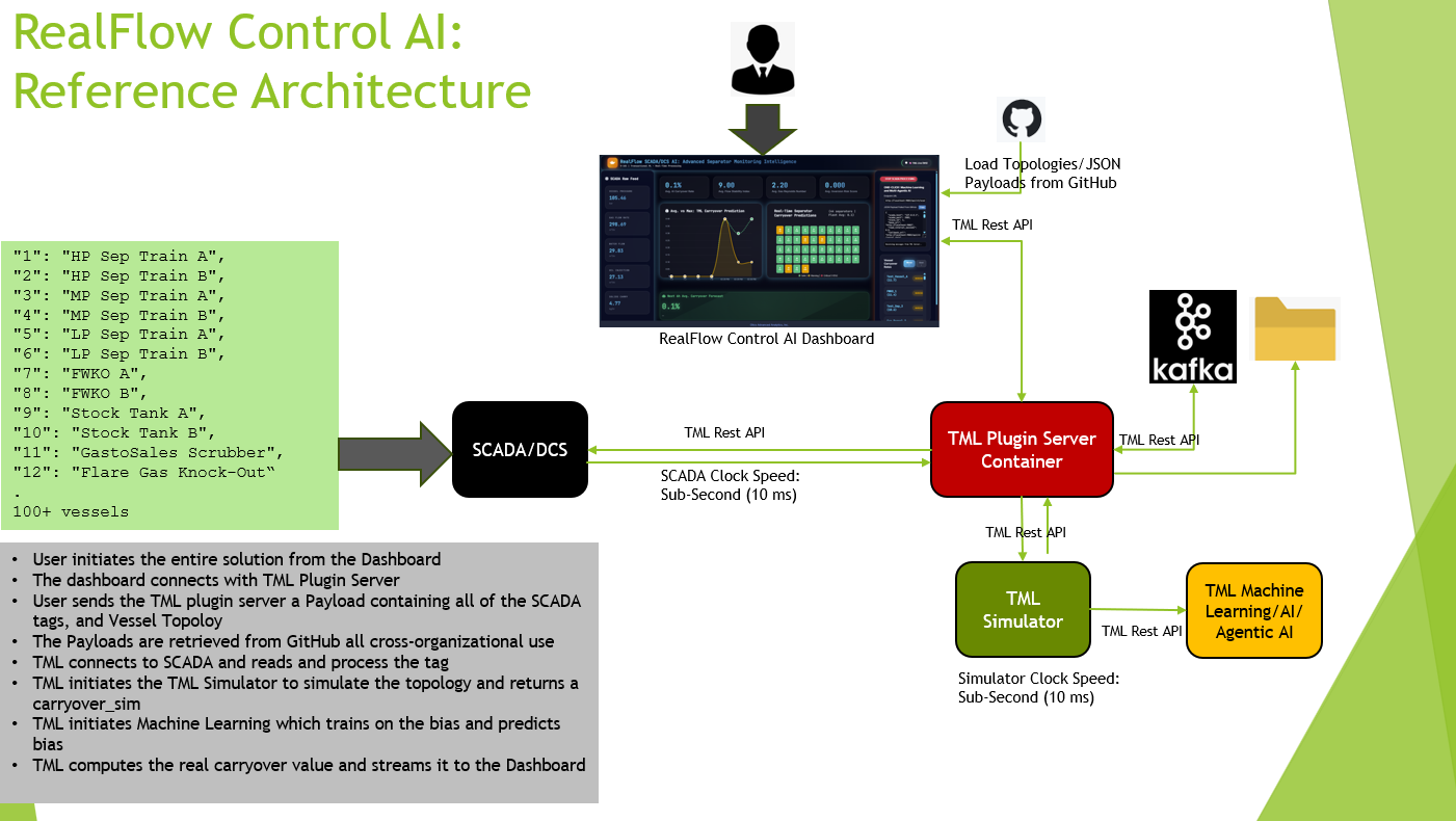
21.6. TML Simulator Solution Reference Architecture

The TML simulator is integrated with SCADA/DCS and integrated with real-time TML, AI and Agentic AI right from the dashboard.

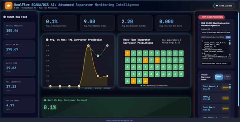
21.7. TML RealFlow Control AI Solution

The TML simulator is integrated with the TML RealFlow Control AI Dashboard.

21.8. Standard Vessel Configuation Template for TML Simulator

Users must provide the following configuration in JSON that is consistent with this template:

   "vessels": [ { ... } ],

   "flows": [ { ... } ],

   "solver": { ... },

   "physics": { "g": 9.81 },

"sendtotopic": "<enter name for kafka topic>",

"topologyname": "<enter topology name>",

"localfoldername": "<enter folder name>"

   }

Example configurations can be found here: https://github.com/smaurice101/raspberrypi/tree/main/tml-airflow/data/payloads/scadaai/carryover
vessels: one entry per vessel, with id, name, type, and V0 (plus any extra‑accurate properties if you want).
flows: one entry per internal flow (from one vessel to another), with from, to, F_in, f_gas.
solver: t0, t_end, dt for design‑mode physics.
physics.g (gravitational constant).

This is sufficient for us to run a SCADA‑baseline carryover‑simulator on your train, and we can handle any number of vessels, any topology, and any outlet‑style flows.”

That’s a clean, global, “Anyone‑Can‑Use‑This” standard that fits your code exactly.

“sendtotopic”: Kafka topic name – all simulation data will be stored in this topic and can be retrieved
“topologyname” : give a name for your topology
“localfoldername” : all simulation data will be stored on a localfolder in CSV format for analysis

21.8.1. 1. vessels — “every vessel matters”

Each vessel must have:

id
name
type (used for physics defaults)
V0 (initial hold‑up volume)
Geometric and physical properties that your VESSEL_PHYSICS can fill in if missing.

"vessels": [

{

"id": 1,

"name": "HP Sep 1A",

"type": "separator",

"V0": 8.0,

"diameter": 3.8,

"height": 15.0,

"rho_l": 880.0,

"rho_g": 70.0,

"mu_g": 1.7e-5,

"inlet_eff": 0.6,

"mist_eff": 0.98,

"souders_k": 0.36,

"gravity_h": 3.0,

"d_mean_um": 250.0,

"d_sigma_um": 1.4,

"carryover_scale": 1.0

},

{

"id": 2,

"name": "HP Sep 1B",

"type": "separator",

"V0": 8.0

},

{

"id": 3,

"name": "MP Sep 1A",

"type": "separator",

"V0": 6.0

},

{

"id": 4,

"name": "MP Sep 1B",

"type": "separator",

"V0": 6.0

},

{

"id": 5,

"name": "LP Sep 1A",

"type": "separator",

"V0": 4.0

},

{

"id": 6,

"name": "LP Sep 1B",

"type": "separator",

"V0": 4.0

},

{

"id": 7,

"name": "FWKO 1A",

"type": "fwko",

"V0": 2.0

},

{

"id": 8,

"name": "FWKO 1B",

"type": "fwko",

"V0": 2.0

},

{

"id": 9,

"name": "Stock Tank 1A",

"type": "tank",

"V0": 6.0

},

{

"id": 10,

"name": "Stock Tank 1B",

"type": "tank",

"V0": 6.0

},

{

"id": 11,

"name": "GastoSales Scrubber",

"type": "separator",

"V0": 1.5

},

{

"id": 12,

"name": "Flare Gas KO",

"type": "separator",

"V0": 1.0

}

]

21.8.2. 2. flows — “every internal pipe”

Each flow must have:

from_id
to_id
F_in (total flow rate in consistent units, e.g., m³/h)
f_gas (gas‑fraction, 0–1)

"flows": [

{ "from": 1, "to": 3, "F_in": 12.0, "f_gas": 0.60 },

{ "from": 2, "to": 4, "F_in": 11.0, "f_gas": 0.60 },

{ "from": 3, "to": 5, "F_in": 8.0, "f_gas": 0.55 },

{ "from": 4, "to": 6, "F_in": 7.5, "f_gas": 0.55 },

{ "from": 5, "to": 7, "F_in": 6.0, "f_gas": 0.50 },

{ "from": 6, "to": 8, "F_in": 6.5, "f_gas": 0.50 },

{ "from": 7, "to": 9, "F_in": 12.0, "f_gas": 0.10 },

{ "from": 8, "to": 10, "F_in": 12.5, "f_gas": 0.10 },

{ "from": 5, "to": 11, "F_in": 3.0, "f_gas": 1.00 },

{ "from": 6, "to": 11, "F_in": 3.2, "f_gas": 1.00 },

{ "from": 11, "to": 0, "F_in": 6.2, "f_gas": 1.00 },

{ "from": 12, "to": 0, "F_in": 0.8, "f_gas": 1.00 }

]

21.8.3. What every company must provide per flow:

from and to (matching existing vessel ids for internal flows)
F_in (total flow rate)
f_gas (gas‑fraction)

If they want to model outlets (e.g., “to sales”, “to flare”), they can:

Use to: 0 (or any id not in vessels) and let the simulator silently ignore them in the internal‑matrix, or
Add a dummy vessel (e.g., id=0, name=”GasToSales”) and treat it like any other node.

Either way, the standard requirement is only to list all internal flows; outlets are optional extras.

21.8.4. 3. solver — “run time range”

This is required for run (design‑mode); run_snapshot can ignore it.

"solver": {

"t0": 0.0,

"t_end": 15.0,

"dt": 0.1

}

21.8.5. What every company must provide:

t0 (start time, usually 0.0)
t_end (end time, e.g., 15.0 hours or 24.0 hours)
dt (time step for design‑mode runs, e.g., 0.1 s)

They can choose:

COARSE mode: dt = 0.1 for fast physics, or
FINE mode: smaller dt, longer t_end.

21.8.6. 4. physics — “global constants”

"physics": {

 "g": 9.81

 }

At a minimum, every company must provide g (gravitational acceleration).

You can extend this later with:

P_gas_ref, T_gas_ref, or other global defaults.

But for now, g is the only absolute requirement.

21.8.7. 5. Minimal “anything‑goes” version

To make it super easy for any company to get started, you can accept a minimal config like this:

{

"vessels": [

{ "id": 1, "name": "Separator 1", "type": "separator", "V0": 10.0 },

{ "id": 2, "name": "FWKO 1", "type": "fwko", "V0": 5.0 },

{ "id": 3, "name": "Stock Tank 1", "type": "tank", "V0": 8.0 }

],

"flows": [

{ "from": 1, "to": 2, "F_in": 10.0, "f_gas": 0.6 },

{ "from": 2, "to": 3, "F_in": 8.0, "f_gas": 0.1 }

],

"solver": { "t0": 0.0, "t_end": 10.0, "dt": 0.1 },

"physics": { "g": 9.81 },

"sendtotopic": "carryover_physics",

"topologyname": "config2",

“localfoldername”: “mysimulationdata”

}

Everything else can be filled from defaults (VESSEL_PHYSICS); they just need to give:

Vessels with id, name, type, V0,
Flows with from, to, F_in, f_gas,
solver time‑range,
physics.g.
sendtotopic : sends this result to a kafka topic
topologyname: give a name to this topology to keep track
localfoldername: stores simulation data to disk

21.8.7.1. **

22. Mapping the SCADA Tags To Vessel Physics

“We need per‑vessel SCADA‑tags:

operatingPressure, operatingTemperature,
gasFlowRate, gasDensity, gasViscosity,
hclFlowRate, hclDensity, hclViscosity,
waterFlowRate, waterDensity, waterViscosity.

From these, we compute:
Total liquid flow,
Gas‑fraction,
rho_l, rho_g, mu_g,
And build an internal flows topology that matches the train‑diagram.
We then run our physics‑engine at SCADA‑frequency and write carryover‑% per vessel back as new tags.”

Below is a direct, field‑ready integration plan based on your:

List of fields (SCADA tags),
The existing PhysicsCarryover engine,
And SCADA / Modbus / OPC‑UA‑style drivers.

22.1. 1. What the SCADA fields give us:

Your fields list is per‑vessel or per‑flow; for each vessel in the train, you typically get:

Operating conditions:
- vesselIndex,
- operatingPressure,
- operatingTemperature.
Gas‑stream:
- gasFlowRate,
- gasDensity,
- gasCompressabilityFactor,
- gasViscosity.
Liquid‑phases:
- hclFlowRate, hclDensity, hclViscosity, hclSurfaceTension,
- waterFlowRate, waterDensity, waterViscosity, waterSurfaceTension,
- hclWaterSurfaceTension,
- phseInversionCriticalWaterCut.
Solids:
- solidFlowRate, solidDensity.

From that, you can construct for each vessel:

Total liquid flow = hclFlowRate + waterFlowRate.
Total liquid density (approx): weighted‑average of hclDensity and waterDensity.
Total liquid viscosity (approx): log‑mean or simple average of hclViscosity and waterViscosity.
Gas‑fraction:
- f_gas = gasFlowRate / (gasFlowRate + totalLiquidFlowRate).
rho_l and rho_g = hcl/water and gasDensity as‑reported.
mu_g = gasViscosity.
F_in_total = gasFlowRate + totalLiquidFlowRate.

You can ignore:

solidFlowRate, solidDensity (for now, unless you want to model sand‑enhanced‑carryover later),
gasCompressabilityFactor (if you’re not doing rigorous EoS corrections).

22.2. 2. Mapping SCADA tags to physics inputs

For each SCADA cycle, for each vessel:

# Example mapping per vessel (inside your SCADA‑loop)

**def** build_vessel_physics_from_tags(vessel_tags):

*# Assume vessel_tags is a dict from SCADA*

P = vessel_tags["operatingPressure"] *# Pa or bar*

T = vessel_tags["operatingTemperature"] *# °C or K*

Fg = vessel_tags["gasFlowRate"] *# m³/s or equivalent*

F_o = vessel_tags["hclFlowRate"] *# oil / HCL*

F_w = vessel_tags["waterFlowRate"] *# water*

rho_g = vessel_tags["gasDensity"]

rho_o = vessel_tags["hclDensity"]

rho_w = vessel_tags["waterDensity"]

mu_g = vessel_tags["gasViscosity"]

*# Compute total liquid flow*

F_l = F_o + F_w

rho_l = (F_o \* rho_o + F_w \* rho_w) / (F_o + F_w) *# vol‑avg*

*# Gas‑fraction in mixed‑flow (use this for your SolverConfig flows)*

**if** F_g + F_l > 0:

f_gas = F_g / (F_g + F_l)

**else**:

f_gas = 0.0

*# Optional: compute liquid‑viscosity log‑mean*

*# mu_l = ... if you want, but not used by your current kernel*

**return** {

"F_in": F_g + F_l, *# m³/s*

"f_gas": f_gas,

"rho_l": float(rho_l),

"rho_g": float(rho_g),

"mu_g": mu_g,

}

Then for each train:

Build flows with from ↔ to and the above F_in, f_gas per vessel.
Build vessels with rho_l, rho_g, mu_g pulled from tags (or from VESSEL_PHYSICS if you prefer fixed defaults).

22.2.1. CORE Mappings For Each Vessel

F_in
f_gas
rho_l
rho_g
mu_g

22.2.1.1. **

22.3. What TML Carryover Solution is Predicting

TML is computing and predicting: “Physics‑baseline + TML bias correction”,

where the real, final carryover the customer cares about is:

\(\text{Carryover}_{\text{real}} = \text{Carryover}_{\text{physics}} + \text{Bias}_{\text{TML}}\)

Here’s how to structure it cleanly.

1. Three carryover quantities

Users track:

carryover_empirical

→ Carryover computed SCADA data:
- carryover_empirical = (waterFlowRate + hclFlowRate + solidFlowRate) / (waterFlowRate + hclFlowRate + solidFlowRate + gasFlowRate)
- raw_co = (waterFlowRate + hclFlowRate + solidFlowRate) / (waterFlowRate + hclFlowRate + solidFlowRate + gasFlowRate)
- TML uses: carryover_empirical = 15.0 * (raw_co ** 0.3)
- “The 15.0 * (raw_co ** 0.3) formula was developed by field operators to:
- Match their observed compressor trips, foamouts, and mist pad inspections
- Provide actionable carryover risk on the dashboard they already trust
- Compress liquid fraction (0-1) into carryover scale (1-15%)
- 15.0 = scaling factor to match field-observed carryover events
- 0.3 exponent = diminishing returns (high liquid load → less marginal carryover risk)
- Validated against: operator experience, upset events, maintenance records
  - 1. Range compression: raw_co^0.3 maps [0,1] → [0,1] with diminishing returns
  - raw_co = 0.1 → 0.46, raw_co = 0.9 → 0.97 (matches carryover behavior)
  - 2. Scale factor 15.0 brings output to 1-15% range (field-observed carryover)
  - 3. Nonlinearity captures physics reality: carryover doesn’t scale linearly with liquid load

SCADA → TML Physics → ML Bias Correction → carryover_final

Legacy: 15.0 * (raw_co ** 0.3) [Operator proxy]

Physics: PhysicsCarryover [First principles]

To ensure we have an Apples-Apples comparison between carryover from SCADA and Physics, the SCADA carryover is scaled using: scaling_factor = carryover_physics/carryover_scada

This creates a new scaled SCADA variable: carryover_scada_norm = carryover_scada * scaling_factor

Bias: ML(carryover_scada_norm - carryover_physics)

Final: carryover_physics + ML_bias [Best of both]

carryover_physics from TML simulator

→ your TML physics‑carryover (%) from PhysicsCarryover (baseline, physically interpretable).
carryover_bias

→ empirical “error” of physics vs empirical (or vs field‑data):

\[\text{carryover_bias} = \text{carryover_scada_norm} - \text{carryover_physics}\]

TML trains and predicts carryover_bias from features:

carryover_bias = f(gasFlowRate, waterFlowRate, operatingPressure, stokes_number, density_ratio, emulsion_ratio, inversion_risk, …)

finally compute the “real” customer‑carryover as:

\[\text{carryover_real} = \text{carryover_physics} + \text{TML_bias_prediction}\]

This is exactly the “bias‑correction” pattern used in climate, CFD, and reservoir‑simulation:

Keep a physics‑baseline model that is interpretable,
Use data to learn the systematic error / bias (foam, slugging, calibration‑drift, etc.),
Combine them into a final prediction that matches field‑experience.

22.4. 2. Why this is better than using only the empirical or only the physics

Only carryover_empirical

→ arbitrary, hard‑to‑explain, hard‑to‑audit.
Only carryover_physics

→ physically sound, but may under‑/over‑estimate real‑world carryover due to:
- Foam,
- Internals,
- Sensor‑calibration,
- Approximations in Souders‑Brown / mist‑pad‑efficiency.
carryover_physics + TML_bias_prediction

→ best of both worlds:
- Physics‑anchor (safety‑related, auditable, can be used for design),
- ML‑correction that adapts to real‑world conditions, foaming‑regimes, and operator‑experience.

→ This is what we show to operators, dashboards, and alarms.

22.4.1. 3. Practical “deployment stages” you can document

3‑stage story:

Stage 1 – Physics‑baseline only
- carryover_physics runs, compared to carryover_empirical (normalized) and field‑data.
- Tunes TML‑physics‑parameters (mist_eff, souders_k, carryover_scale) until baseline is sensible.
Stage 2 – Physics‑baseline + bias‑learning
- Fit ML to (empirical_normalized – physics) = bias,
- Show that ML‑bias‑correction reduces residuals versus field‑data.
Stage 3 – Full “real carryover” layer
- Operators see carryover_real = physics + ML‑bias,
- Explainable: “physics says X, ML‑correction adds Y due to foam / slugging / calibration‑drift.”

This is key to:

Operators: “We have a real‑physics‑anchor, not just a black‑box formula.”
Engineers / auditors: “You can inspect the baseline and validate it against Aspen‑style tools.”
Executives: “We’re using ML to refine first‑principles physics, not replace it.”

22.4.2. Summary

We Do This:

Compute carryover_physics (TML),
Compute carryover_empirical (legacy formula) and normalize to carryover_scada_norm,
Define carryover_bias = carryover_scada_norm − carryover_physics,
Train ML to predict carryover_bias,
Then report:

\[\boxed{\text{carryover_real}\mathbf{=}\text{carryover_physics}\mathbf{+}\text{TML_bias_prediction}}\]

That gives you a production‑ready, physics‑anchored, ML‑corrected carryover‑engine that every oil‑and‑gas company will understand and trust.

22.5. Vessel Configuration: Example of 20 Vessels

Goto Github to see configuration in section “tml_physics_simulator”: https://github.com/smaurice101/raspberrypi/blob/main/tml-airflow/data/payloads/scadaai/carryover/config20

22.6. Vessel Configuration: Example of 150 Vessels

Goto Github to see configuration in section “tml_physics_simulator”: https://github.com/smaurice101/raspberrypi/blob/main/tml-airflow/data/payloads/scadaai/carryover/config150

22.7. TML RealFlow Solution

The entire physics-based model and SCADA/DCS integration is triggered directly from the TML RealFlow dashboard shown below.

22.8. Customers’ Advantages:

Worlds FASTEST and direct physics-based simulator that directly uses SCADA data in real-time for the Physics integrated with real-time machine learning, AI, Agentic AI
Low-cost – no PI Historian needed – Physics simulator bundled in the Dashboard.
Scalable across complex topologies and configurations
Dashboard driven – minimal training required.
All data: simulation, machine learning and AI stored on Apache Kafka topic, and on local disk in CSV and JSON
Complete transparency and auditability
Engineer / Data Scientist Focused with the Business in Mind

23. 1D Souders-Brown and 3D CFD

1D Souders-Brown is a fast empirical equation for separator design, while full 3D CFD provides detailed flow visualization but at much higher computational cost.

23.1. Core Physics Approach

Souders-Brown (1D):

\[Vs = K \* sqrt( (ρL - ρG) / ρG )\]

Assumptions:

Uniform gas velocity across vessel cross-section, no wall effects, droplets follow Stokes settling
What it predicts: Maximum allowable superficial gas velocity before liquid carryover
Dimensions: Single velocity value (scalar) per vessel
Runtime: Milliseconds

3D CFD (CFF/Computational Fluid Dynamics):

Solves full Navier-Stokes equations across vessel mesh (10k-10M cells)
Captures velocity gradients, recirculation zones, inlet jetting, wall wetting
Outputs full 3D velocity/pressure/droplet concentration fields
Runtime: Hours-days

Practical Differences

Aspect	1D Souders-Brown	3D CFD
Geometry	Diameter only	Full CAD vessel + internals
Flow Field	Uniform velocity	3D velocity vectors + turbulence
Droplet Tracking	Population balance (your code)	Lagrangian particle tracking
Validation	Field data correlations	Lab experiments + field
Use Case	Vessel sizing, screening	Troubleshooting carryover, optimization
Your Code	Implements this exactly	N/A

23.2. When Each Wins: 1D vs 3D

Use 1D Souders-Brown (your simulator):

Vessel networks (100+ vessels)
Real-time SCADA bias correction
Parametric studies (what-if sizing)
Daily operations monitoring

Use 3D CFD:

Single problem vessel with unexpected carryover
New internals design (mist pads, baffles)
Inlet device optimization
CFD validates your 1D assumptions

23.3. Hybrid Reality (Industry Practice)

Most operators run 1D physics → flag vessels >2-3% carryover → run 3D CFD on those specific vessels only.

TML Simulator sophisticated: quadrature droplet distribution + Souders mist loading.

The Souders-Brown in your PhysicsCarryover is production-grade for fleet monitoring.
3D CFD would be for the 5% of vessels that fail your screen.

Perfect architecture.

23.4. Industry Perspective

1D Souders-Brown remains excellent for production use—it’s been the oil & gas industry standard for 80+ years for good reason.

Why It’s Still “Very Good”

1. Field-Proven Accuracy

Correctly sizes 90%+ of separators worldwide
TML simulation mist loading + quadrature droplets makes it more sophisticated than basic Vs equation
Validates against decades of operational data across thousands of vessels

23.5. Computational Reality

TML Simulator uses Numba code: ~1ms per snapshot (100 vessels)
- Numba code is Python code accelerated by the Numba JIT (Just-In-Time) compiler.

@njit(fastmath=True) # ← This decorator = Numba magic

def physics_carryover(…):

# NumPy loops → C-speed machine code

Without Numba:

100 vessels × 24hr sim = 10+ seconds per call → Too slow for SCADA

With Numba (TML Simulator):

100 vessels × 24hr sim = 1-10ms → Perfect for real-time flowsheet

Full 3D CFD: ~24+ hours per vessel

You can run your physics 86 million times in the same time CFD takes for one vessel.

23.6. Network Scale

Single vessels: CFD occasionally beats 1D by 5-10%
Fleet monitoring (TML use case): 1D physics catches the 5% problem vessels perfectly
CFD can’t economically screen 100+ vessels daily

23.7. Engineering Truth

Souders-Brown + your droplet distribution + mist efficiency = production-grade physics that pays for itself daily through avoided carryover losses.
CFD is for the edge cases your code correctly identifies.

23.8. Carryover Details

SCADA carryover IS per-vessel and physics accounts for topology coupling:

SCADA carryover field = measured outbound carryover per vessel i.
Physics carryover[:,i] = predicted outbound carryover for vessel i.
Carryover_bias = measured (from SCADA) – predicted (from Physics) (per vessel – directly comparable)

Details:

Carryover_scada = 15.0 * (raw_co ** 0.3) (this equation can be changed by user)

This value is calculated for every SCADA data generated by the vessels – it is NOT using the Physics simulator – it’s a straightforward calculation

absolute carryover (kg/s)

it is computed for each vessel -so 12 vessels – 12 carryover_scada calculations each time new data shows up in SCADA

SCADA measures OUTBOUND carryover per vessel

Each sensor sees its vessel’s carryover

carryover_physics :

This DOES use the TML simulator physics (with Step=1, steady state) using the customer provided topology (i.e.config2)

Physics simulates the SAME per-vessel carryover using the SAME SCADA data as in carryover_scada in its topology

EXAMPLE:

Vessel 1 (HP Sep):

o SCADA: fg_tot=370 kg/h → carryover_scada = 0.00089 kg/s ✓

o Physics: fg_tot=370 kg/h → carryover_physics = 0.000010 kg/s ✓

o Bias: 0.00089 - 0.000010 = 0.00088 kg/s

23.9. Flowsheet: 1D Souders-Brown and 3D CFD

Flowsheet Architecture

Aspect*	TML 1D Souders-Brown	3D CFD
Scope	Multi-vessel network (HP → IP → LP separators, FWKO, tanks)	Single vessel internals
Nodes	50-200 vessels + flows	1 vessel (10M+ mesh cells)
Conn ections	Flow matrices (gas/liquid streams)	Inlet/outlet boundary conditions
Physics	Per-vessel carryover %	3D vel ocity/turbulence/droplet fields
Solve Time	1-10ms total network	12-72hrs per vessel

23.10. Units Table

Variable	Likely Units / Scaling Explanation
vesselIndex	unitless index (integer 1–12)
operatingPressure (Pg)	bar or psig (SCADA‑scaled; treat as absolute pressure in bar if using SI)
operatingTemperature	°C
gasFlowRate (Qg)	kg/s or m³/s (mass or volumetric gas rate)
gasDensity (rhog)	kg/m³ (gas density, but 0.0 here is invalid / bad signal)
g asCompressabilityFactor (Zg)	unitless, scaled as Zg = Z×1000 (so 960 → 0.960)
gasViscosity (mug signal)	Raw SCADA value; your derived mug = gasViscosity / 1000000.0 should be Pa·s (≈ cP scaled to SI)
hclFlowRate (Qh)	kg/s or m³/s (acid / liquid flow)
hclDensity (ρh)	kg/m³
hclViscosity	cP‑like / scaled viscosity; treat as mPas or Pa·s depending on context
hclSurfaceTension (sow)	mN/m or dyne/cm (surface tension liquid–liquid)
waterFlowRate (Qw)	kg/s or m³/s (water flow)
waterDensity (rhow)	kg/m³ (≈1000 kg/m³ for water)
waterViscosity (muw signal)	Raw SCADA value; derived muw should be Pa·s
waterSurfaceTension (sw)	mN/m or dyne/cm (surface tension liquid–gas)
hclWaterSurfaceTension (sow)	mN/m or dyne/cm (liquid–liquid surface tension)
phseIn versionCriticalWaterCut	unitless fraction × 1000, e.g., 444 → 0.444 (44.4%)
picwc	unitless fraction (critical water cut)
solidFlowRate (Qs)	kg/s or m³/s (solid flow)
solidDensity	kg/m³ (≈100–3000 kg/m³ depending on solids)
rho_l	kg/m³ (total liquid density, derived from mixing rule)
raw_co	unitless fraction (0–1) of liquid vs total phase
carryover	This is a scaled index (e.g., carryover = 15.0 * (raw_co*0.3)); after normalization with carryover_scada_norm = carryover scaling_factor, it becomes physical carryover (kg/s, or same unit as your physics baseline) The Scaling factor is simple: scaling_factor = carryover_sim/carryover Carryover_bias = carryover_scada_norm – carryover_sim
flow_stability	unitless or engineering index (high values indicate instability)
F_liq	kg/s or m³/s (total liquid flow: Qw + Qh + Qs)
F_total	kg/s or m³/s (total in‑going flow, Qg + F_liq)
gas_reynolds	Re = (Qg × rhog) / (mug + 1e-6) → dimensionless (gas Reynolds)
Qs	kg/s or m³/s (same as above; duplicated for access)
emulsion_ratio (sw / sow)	unitless (surface tension ratio, liquid–gas vs liquid–liquid)
reynolds_ratio	unitless (Re_gas / Re_water)
f_gas	unitless fraction (gas fraction of total flow)
muw	Pa·s (water viscosity, derived)
sw	mN/m or dyne/cm (surface tension, same as above)
rhow	kg/m³ (same as above)
inversion_risk	unitless index (Qw / Qg − picwc)
density_ratio (rhow / rhog)	unitless (liquid/gas density ratio)
water_reynolds	Re_water = (Qw × rhow) / (muw + 1e-6) → dimensionless
Qw	kg/s or m³/s (same as above)
stokes_number	unitless (classical or system‑defined Stokes‑number‑like term)
Qg	kg/s or m³/s (same as above)
Pg	bar or psig (same as operatingPressure)
Qh	kg/s or m³/s (same as above)
mug	Pa·s (gas viscosity, derived from gasViscosity scaled)
sow	mN/m or dyne/cm (same as above)
Zg	unitless compressibility factor, derived as Zg = gasCompressabilityFactor / 1000.0

23.11. Vessel and Model Variables

23.11.1. Scada Raw Measurements

Variable	U nit s	Scale Fac tor	Importance*	Role
o peratingPressure (Pg)	p sig	/100	Vessel operating condition	Drives gas density, compressibility, Souders velocity
oper atingTemperature (T)	°F	/100	Thermodynamic state	Affects all fluid properties (rho, mu, Z)
gasFlowRate (Qg)	k g/h	/100	Primary separation driver	Determines gas velocity → carryover
waterFlowRate (Qw)	k g/h	/1000	Liquid loading	Flooding risk, phase inversion
hclFlowRate (Qh)	k g/h	/100	Oil/HCl flow	Liquid density, total F_liq
solidFlowRate (Qs)	k g/h	/100	Solids carryover	Erosion, fouling risk

23.12. Fluid Properties

Variable	U nit s	Scale Fac tor	Im portance	Role
gasDensity (rhog)	kg /m³	/1000	Gas momentum	Gas Re# → entrainment
waterDensity (rhow)	kg /m³	/10	Buoyancy force	Stokes settling velocity
gasViscosity (mug)	P a·s	/1e8	Drag forces	Droplet Reynolds number
waterViscosity (muw)	P a·s	/1e6	Liquid drag	Liquid film stability
waterSurfaceTension (sw)	N/m	/1e5	Emulsion stability	Inversion risk
hclWaterSurfaceTension (sow)	N/m	/1e5	Interface tension	Emulsion ratio
gasCompressabilityFactor (Zg)		/1000	Real gas behavior	Accurate rho_g = PM/ (ZRT)
phse InversionCriticalWaterCut (picwc)	f rac	/1000	Emulsion threshold	Phase inversion risk

23.13. Physics/Derived

Va riable	U nit s	Source*	Importance	Role
F_liq	k g/h	Qh+Qw+Qs	Liquid holdup	Level control, flooding
rho_l	kg /m³	Weighted	Liquid momentum	Liquid Re#, entrainment
F_total	k g/h	Qg+F_liq	Total throughput	Vessel capacity
f_gas	F rac	Q g/F_total	Phase ratio	Gas velocity scaling
hu[i]	M	vol/(ar eaht)	Liquid level	Gas space volume
f g_tot[i]	k g/h	Σ(fg_m athu)	Vessel gas load	Primary carryover driver
f l_tot[i]	k g/h	Σ(fl_m athu)	Vessel liquid load	Level dynamics
gvol[i]	m³	are a*(ht-hl)	Gas disengagement	gvel = fg_tot/gvol
gvel[i]	m/s	fg/ 3600/gvol	Gas velocity	Souders-Brown core
carr yover[i]	F rac	Physics	Prediction	ML bias training target

23.14. Simulator Arrays

Array	Sh ape	Uni ts*	Im portance	Role
areas[i]	(12,)	m²	Geometry	Level → hl = vol/area
hts[i]	(12,)	m	Geometry	Gas height = ht-hl
ein[i]	(12,)	frac	Inlet sep	Primary separation
vs_souders[i]	(12,)	m/s	Design limit	K√[(ρl-ρg)/ρg]
em[i]	(12,)	frac	Mist pad	Secondary entrainment
car ryover_scale[i]	(12,)		C alibration	Physics → SCADA match
f_gas_mat	(1 2,12)	kg/h	Flow routing	HP→MP→LP topology
carryover[t,i]	( N,12)	frac	Output	Real-time predictions

23.15. Analytics Features

Variable	U nit s	Formula	Im portance	Role
raw_co	f rac	(Q w+Qh+Qs)/F_total	Ground truth	ML training target
gas_reynolds		ρggvelD/μg	Flow regime	Tur bulent/laminar
wa ter_reynolds		ρ lv_liqD/μl	Liquid regime	Film stability
s tokes_number		( ρl-ρg)μl/Pg²	Droplet sep	Settling efficiency
in version_risk		(Qw/Qg)-picwc	Emulsion risk	Operational alert
em ulsion_ratio		sw/sow	Stability	Coalescence rate

23.16. Payload Key Fields

The following table describes the main configuration keys.

Field name	Role / meaning
`scada_host`	Host IP (or hostname) of the SCADA/Modbus source to read from (here `127.0.0.1`).
`scada_port`	Port number on the SCADA host for Modbus‑TCP or similar polling (here `2502`).
`slave_id`	Modbus slave ID of the device/PLC inside the SCADA network.
`base_url`	Base HTTP endpoint for services (e.g., internal APIs or dashboards).
`read_interval_seconds`	Polling interval (in seconds) between SCADA reads; `0.5` = 500 ms.
`callback_url`	Webhook URL (in this block) to POST processed data or alerts; empty means no callback.
`max_reads`	Limit on read cycles; `-1` means unlimited / continuous polling.
`start_register`	Starting Modbus register address (e.g., `40001`) from which raw values are read.
`sendtotopic` (raw)	Kafka / messaging topic name for raw SCADA‑style data; here `scada-raw-data`.
`createvariables`	Inline expression string defining derived physics variables (e.g., `carryover`, `F_total`, `emulsion_ratio`, etc.).
`fields`	List of variable names (e.g., `gasFlowRate`, `operatingPressure`) read from SCADA and used in calculations.
`scaling`	Maps each field to a scaling factor (e.g., `gasCompressabilityFactor` scaled by `1000`) for unit‑matching.
`vessel_names`	Dictionary mapping integer IDs to human‑readable vessel names (e.g., `"1": "HP Sep Train A"`).
`carryover_topology`	Sub‑object describing vessel geometry, flow connections, and physics parameters for carryover modeling.
`sendtotopic` (physics)	Topic name for physics‑enriched carryover data; here `carryover_physics`.
`topologyname`	Name / tag of this configuration/topology (e.g., `config12`) used for logging or file‑system naming.
`localfoldername`	Local disk folder where to store intermediate/output data (here `mycarryoverdata`).
`rollbackoffsets`	Number of Kafka message offsets to roll back when re‑processing physics (here `300`).
`time_interval`	Time interval (in seconds) between execution or data‑ bundle events in the physics pipeline (here `5`).
`preprocessed_physics_topic`	Kafka topic name for SCADA‑plus‑physics data after preprocessing (here `scada_with_physics`).
`savetodiskfrequency`	Frequency (or period) for saving to disk; `0` likely means “no periodic save” or event‑driven.
`carryoverthreshold`	Threshold on carryover (e.g., in kg/s or scaled units) above which an alert or special path is triggered (here `0.015`).
`alertemails`	Comma‑separated email list to notify when thresholds are breached; empty here means no email alerts.
`preprocessing`	Config block for pre‑processing steps (windowing, JSON criteria, source/destination topics, etc.).
`machinelearning`	ML block: training folder, topics, dependent/independent variables, and rolling‑window parameters.
`predictions`	Prediction‑stage config: source topic, input streams, model path, and output topic for ML predictions.
`agenticai`	Block for agentic‑style orchestration (step `9b` in your workflow).
`ai`	Higher‑level AI / orchestration step (`9`) in the overall pipeline.
`validation_bounds`	Allows users to specify a bounds for the raw SCADA data. Bad data at source, will impact downstream analysis.